Hello, world! This week in Advanced Statistics and Analysis we covered regression analysis. The first question for this week is as follows: 

1.1 Define the relationship model between the predictor and the response variable:
1.2 Calculate the coefficients.

This is the data set we will be using for this question:

x <- c(16, 17, 13, 18, 12, 14, 19, 11, 11, 10)
y <- c(63, 81, 56, 91, 47, 57, 76, 72, 62, 48)

The predictor variable is y, and is used to predict the response variable x. So in this problem, we will be searching for how y changes relative to changes in x. To begin, I made a simple plot of the existing data to aid in visualization. 

Based on this graph, there appears to be a positive, linear relationship between x and y. I then used the following R code to perform a linear regression:

#Stores the dataset in their variables
x <- c(16, 17, 13, 18, 12, 14, 19, 11, 11, 10)
y <- c(63, 81, 56, 91, 47, 57, 76, 72, 62, 48)
#Fits a linear regression 
lm(y ~ x)

When this code is run, it returns an intercept of 19.205597 and a regression coefficient of 3.269107. Here’s the complete output generated by R:

Call:
lm(formula = y ~ x)

Residuals:

    Min      1Q  Median      3Q     Max 

-11.435  -7.406  -4.608   6.681  16.834 

Coefficients:

            Estimate Std. Error t value Pr(>|t|)
  
(Intercept)   19.206     15.691   1.224   0.2558  

x               3.269      1.088   3.006   0.0169 
*
---
Signif. codes:  0 ‘***’ 0.001 ‘**’ 0.01 ‘*’ 0.05 ‘.’ 0.1 ‘ ’ 1


Residual standard error: 10.48 on 8 degrees of freedom
Multiple R-squared:  0.5303,	Adjusted R-squared:  0.4716 

F-statistic: 9.033 on 1 and 8 DF,  p-value: 0.01693

By looking at this output, we can determine that the average value of y when x = 0 is 19.206, and y will increase by 3.269 each time x increases by 1.

On to the next question!

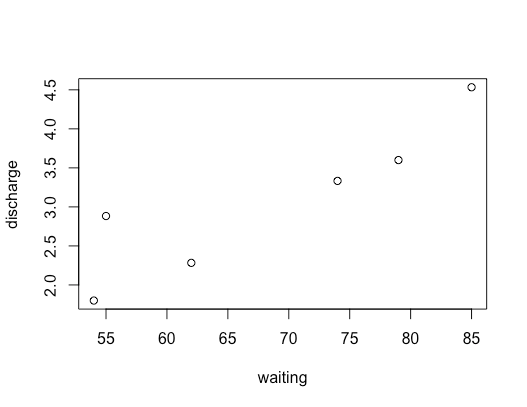
Apply the simple linear regression model (see the above formula) for the data set called “visit” (see below), and estimate the the discharge duration if the waiting time since the last eruption has been 80 minutes.

	discharge	waiting
1	3.600	79
2	1.800	54
3	3.333	74
4	2.283	62
5	4.533	85
6	2.883	55

2.1 Define the relationship model between the predictor and the response variable.
2.2 Extract the parameters of the estimated regression equation with the coefficients function.
2.3 Determine the fit of the eruption duration using the estimated regression equation.

To start off, I made a scatterplot to display our data visually. Using the plot, we can determine that the data has a positive, linear relationship.

To solve this problem, I used the following R code:

#Initialize variables
discharge <- c(3.600, 1.800, 3.333, 2.283, 4.533, 2.883)
waiting <- c(79, 54, 74, 62, 85, 55)

#Store the dataset in a data frame
visit <- as.data.frame(cbind(discharge, waiting))

#Fits a linear regression using discharge as Y and waiting as X 
discharge.lm <- lm(discharge ~ waiting, data = visit)

#Stores the coefficients as a variable
coeffs <- coefficients(discharge.lm)

# Prints the coefficients
coeffs

#Sets the waiting time we're testing for
waiting = 80

#Uses the regression equation with the coefficients from the lm() function
duration <- coeffs[1] + coeffs[2]*waiting

#Prints duration
duration 

In this problem, we are seeking to find out how the discharge variable changes in relation to the waiting variable. Once you print the coefficient variable shown above, R returns an intercept of -1.53317418 and a regression coefficient of 0.06755757, which means that when the wait time is 0, the average discharge time will be -1.533 and when the wait time increases by 1, the duration length will increase by 0.06755757. Since we are testing for how long the discharge duration will be when the waiting time since the last eruption is 80 minutes, I assigned “80” to the variable “waiting.” Using the regression equation and the coefficients determined in our earlier linear regression model, we are able to determine the eruption duration for a wait time of 80 minutes. When we print the duration variable, R returns the intercept value of 3.871431. Therefore, if the waiting period has been 80 minutes, the discharge duration will be 3.871431 minutes. 

For the next question, we will be using R’s mtcars dataset to complete the following problem: 

3.1 Examine the relationship Multi Regression Model as stated above and its Coefficients using 4 different variables from mtcars (mpg, disp, hp and wt).
Report on the result and explanation what does the multi regression model and coefficients tells about the data?   

I used this R code to complete the problem:

#Initialize variables from mtcars
input <- mtcars[,c("mpg", "disp", "hp", "wt")]

#Runs a linear regression analysis on the input dataset for mpg based on disp, hp and wt
mpg.lm <- lm(formula = mpg ~ disp+ hp + wt, data = input)

#Calls mpg.lm
mpg.lm

Calling mpg.lm returns the following output:

> mpg.lm

Call:

lm(formula = mpg ~ disp + hp + wt, data = input)

Coefficients:

(Intercept)         disp           hp           wt  

  37.105505    -0.000937    -0.031157    -3.800891   

From this data, we can see that the intercept is 37.105505. For each mile per gallon, the displacement is shifted by -0.000937, the horsepower is shifted by -0.031157, and the weight is shifted by -3.800891. So, for the car in the dataset to have more miles per gallon, it generally comes at the cost of reduced displacement, horsepower, and weight. 

Next question: 

With the rmr data set, plot metabolic rate versus body weight. Fit a linear regression to the relation. According to the fitted model, what is the predicted metabolic rate for a body weight of 70 kg? 

I used the following R code to complete this question:

#Loads ISwR package
library(ISwR)

#Plots the linear regression of metabolic rate in relation to weight
plot(metabolic.rate~body.weight, data=rmr)

#Assigns linear regression to variable
mr.lm <- lm(metabolic.rate~body.weight, data=rmr)

#Assigns the coefficients of mr.lm to a variable
cf <- coefficients(mr.lm)

#Sets body weight to test for in variable
body.weight <- 70

#Uses the regression equation with coefficients
p.mr <- cf[1] + cf[2] * body.weight

#Prints result
print(p.mr) 

The linear regression for the original call returned an intercept of 811.23 and a regression coefficient of 7.06. When we set the body weight as 70, R returns an intercept of 1305.394. Therefore, when the body weight is 70 we can expect a metabolic rate of 1305.394.

And that’s all for this assignment! See you next week!